Parcels documentation

Welcome to the documentation of parcels. This page provides detailed documentation for each method, class and function. The documentation corresponds to the latest conda release, for newer documentation see the docstrings in the code.

See http://www.oceanparcels.org for general information on the Parcels project, including how to install and use.

parcels.particleset module

parcels.fieldset module

class parcels.fieldset.FieldSet(U, V, fields=None)

Bases: object

FieldSet class that holds hydrodynamic data needed to execute particles

Parameters

• U – parcels.field.Field object for zonal velocity component

• V – parcels.field.Field object for meridional velocity component

• fields – Dictionary of additional parcels.field.Field objects

add_constant(name, value)

Add a constant to the FieldSet. Note that all constants are stored as 32-bit floats. While constants can be updated during execution in SciPy mode, they can not be updated in JIT mode.

Tutorials using fieldset.add_constant: Analytical advection Diffusion Periodic boundaries

Parameters

• name – Name of the constant

• value – Value of the constant (stored as 32-bit float)

add_constant_field(name, value, mesh='flat')

Wrapper function to add a Field that is constant in space,

useful e.g. when using constant horizontal diffusivity

Parameters

• name – Name of the parcels.field.Field object to be added

• value – Value of the constant field (stored as 32-bit float)

• units – Optional UnitConverter object, to convert units (e.g. for Horizontal diffusivity from m2/s to degree2/s)

add_field(field, name=None)

Add a parcels.field.Field object to the FieldSet

Parameters

• field – parcels.field.Field object to be added

• name – Name of the parcels.field.Field object to be added

For usage examples see the following tutorials:

• Nested Fields

• Unit converters

add_periodic_halo(zonal=False, meridional=False, halosize=5)

Add a ‘halo’ to all parcels.field.Field objects in a FieldSet, through extending the Field (and lon/lat) by copying a small portion of the field on one side of the domain to the other.

Parameters

• zonal – Create a halo in zonal direction (boolean)

• meridional – Create a halo in meridional direction (boolean)

• halosize – size of the halo (in grid points). Default is 5 grid points

add_vector_field(vfield)

Add a parcels.field.VectorField object to the FieldSet

Parameters

vfield – parcels.field.VectorField object to be added

advancetime(fieldset_new)

Replace oldest time on FieldSet with new FieldSet

Parameters

fieldset_new – FieldSet snapshot with which the oldest time has to be replaced

computeTimeChunk(time, dt)

Load a chunk of three data time steps into the FieldSet. This is used when FieldSet uses data imported from netcdf, with default option deferred_load. The loaded time steps are at or immediatly before time and the two time steps immediately following time if dt is positive (and inversely for negative dt)

Parameters

• time – Time around which the FieldSet chunks are to be loaded. Time is provided as a double, relatively to Fieldset.time_origin

• dt – time step of the integration scheme

classmethod from_b_grid_dataset(filenames, variables, dimensions, indices=None, mesh='spherical', allow_time_extrapolation=None, time_periodic=False, tracer_interp_method='bgrid_tracer', chunksize=None, **kwargs)

Initialises FieldSet object from NetCDF files of Bgrid fields.

Parameters

• filenames – Dictionary mapping variables to file(s). The filepath may contain wildcards to indicate multiple files, or be a list of file. filenames can be a list [files], a dictionary {var:[files]}, a dictionary {dim:[files]} (if lon, lat, depth and/or data not stored in same files as data), or a dictionary of dictionaries {var:{dim:[files]}} time values are in filenames[data]

• variables – Dictionary mapping variables to variable names in the netCDF file(s).

• dimensions –

  Dictionary mapping data dimensions (lon, lat, depth, time, data) to dimensions in the netCF file(s). Note that dimensions can also be a dictionary of dictionaries if dimension names are different for each variable. U and V velocity nodes are not located as W velocity and T tracer nodes (see http://www.cesm.ucar.edu/models/cesm1.0/pop2/doc/sci/POPRefManual.pdf ).

  U[k,j+1,i],V[k,j+1,i]		U[k,j+1,i+1],V[k,j+1,i+1]
  	W[k:k+2,j+1,i+1],T[k,j+1,i+1]
  U[k,j,i],V[k,j,i]		U[k,j,i+1],V[k,j,i+1]

  In 2D: U and V nodes are on the cell vertices and interpolated bilinearly as a A-grid.

  T node is at the cell centre and interpolated constant per cell as a C-grid.

  In 3D: U and V nodes are at the midlle of the cell vertical edges,

  They are interpolated bilinearly (independently of z) in the cell. W nodes are at the centre of the horizontal interfaces. They are interpolated linearly (as a function of z) in the cell. T node is at the cell centre, and constant per cell.

• indices – Optional dictionary of indices for each dimension to read from file(s), to allow for reading of subset of data. Default is to read the full extent of each dimension. Note that negative indices are not allowed.

• fieldtype – Optional dictionary mapping fields to fieldtypes to be used for UnitConverter. (either ‘U’, ‘V’, ‘Kh_zonal’, ‘Kh_meridional’ or None)

• mesh –

  String indicating the type of mesh coordinates and units used during velocity interpolation:

  1. spherical (default): Lat and lon in degree, with a correction for zonal velocity U near the poles.

  2. flat: No conversion, lat/lon are assumed to be in m.

• allow_time_extrapolation – boolean whether to allow for extrapolation (i.e. beyond the last available time snapshot) Default is False if dimensions includes time, else True

• time_periodic – To loop periodically over the time component of the Field. It is set to either False or the length of the period (either float in seconds or datetime.timedelta object). (Default: False) This flag overrides the allow_time_interpolation and sets it to False

• tracer_interp_method – Method for interpolation of tracer fields. It is recommended to use ‘bgrid_tracer’ (default) Note that in the case of from_pop() and from_bgrid(), the velocity fields are default to ‘bgrid_velocity’

• chunksize – size of the chunks in dask loading

classmethod from_c_grid_dataset(filenames, variables, dimensions, indices=None, mesh='spherical', allow_time_extrapolation=None, time_periodic=False, tracer_interp_method='cgrid_tracer', gridindexingtype='nemo', chunksize=None, **kwargs)

Initialises FieldSet object from NetCDF files of Curvilinear NEMO fields.

See here for a more detailed explanation of the different methods that can be used for c-grid datasets.

Parameters

• filenames – Dictionary mapping variables to file(s). The filepath may contain wildcards to indicate multiple files, or be a list of file. filenames can be a list [files], a dictionary {var:[files]}, a dictionary {dim:[files]} (if lon, lat, depth and/or data not stored in same files as data), or a dictionary of dictionaries {var:{dim:[files]}} time values are in filenames[data]

• variables – Dictionary mapping variables to variable names in the netCDF file(s).

• dimensions –

  Dictionary mapping data dimensions (lon, lat, depth, time, data) to dimensions in the netCF file(s). Note that dimensions can also be a dictionary of dictionaries if dimension names are different for each variable. Watch out: NEMO is discretised on a C-grid: U and V velocities are not located on the same nodes (see https://www.nemo-ocean.eu/doc/node19.html ).

  	V[k,j+1,i+1]
  U[k,j+1,i]	W[k:k+2,j+1,i+1],T[k,j+1,i+1]	U[k,j+1,i+1]
  	V[k,j,i+1]

  To interpolate U, V velocities on the C-grid, Parcels needs to read the f-nodes, which are located on the corners of the cells. (for indexing details: https://www.nemo-ocean.eu/doc/img360.png ) In 3D, the depth is the one corresponding to W nodes.

• indices – Optional dictionary of indices for each dimension to read from file(s), to allow for reading of subset of data. Default is to read the full extent of each dimension. Note that negative indices are not allowed.

• fieldtype – Optional dictionary mapping fields to fieldtypes to be used for UnitConverter. (either ‘U’, ‘V’, ‘Kh_zonal’, ‘Kh_meridional’ or None)

• mesh –

  String indicating the type of mesh coordinates and units used during velocity interpolation:

  1. spherical (default): Lat and lon in degree, with a correction for zonal velocity U near the poles.

  2. flat: No conversion, lat/lon are assumed to be in m.

• allow_time_extrapolation – boolean whether to allow for extrapolation (i.e. beyond the last available time snapshot) Default is False if dimensions includes time, else True

• time_periodic – To loop periodically over the time component of the Field. It is set to either False or the length of the period (either float in seconds or datetime.timedelta object). (Default: False) This flag overrides the allow_time_interpolation and sets it to False

• tracer_interp_method – Method for interpolation of tracer fields. It is recommended to use ‘cgrid_tracer’ (default) Note that in the case of from_nemo() and from_cgrid(), the velocity fields are default to ‘cgrid_velocity’

• gridindexingtype – The type of gridindexing. Set to ‘nemo’ in FieldSet.from_nemo() See also the Grid indexing documentation on oceanparcels.org

• chunksize – size of the chunks in dask loading

classmethod from_data(data, dimensions, transpose=False, mesh='spherical', allow_time_extrapolation=None, time_periodic=False, **kwargs)

Initialise FieldSet object from raw data

Parameters

• data –

  Dictionary mapping field names to numpy arrays. Note that at least a ‘U’ and ‘V’ numpy array need to be given, and that the built-in Advection kernels assume that U and V are in m/s

  1. If data shape is [xdim, ydim], [xdim, ydim, zdim], [xdim, ydim, tdim] or [xdim, ydim, zdim, tdim], whichever is relevant for the dataset, use the flag transpose=True

  2. If data shape is [ydim, xdim], [zdim, ydim, xdim], [tdim, ydim, xdim] or [tdim, zdim, ydim, xdim], use the flag transpose=False (default value)

  3. If data has any other shape, you first need to reorder it

• dimensions – Dictionary mapping field dimensions (lon, lat, depth, time) to numpy arrays. Note that dimensions can also be a dictionary of dictionaries if dimension names are different for each variable (e.g. dimensions[‘U’], dimensions[‘V’], etc).

• transpose – Boolean whether to transpose data on read-in

• mesh –

  String indicating the type of mesh coordinates and units used during velocity interpolation, see also this tutorial:

  1. spherical (default): Lat and lon in degree, with a correction for zonal velocity U near the poles.

  2. flat: No conversion, lat/lon are assumed to be in m.

• allow_time_extrapolation – boolean whether to allow for extrapolation (i.e. beyond the last available time snapshot) Default is False if dimensions includes time, else True

• time_periodic – To loop periodically over the time component of the Field. It is set to either False or the length of the period (either float in seconds or datetime.timedelta object). (Default: False) This flag overrides the allow_time_interpolation and sets it to False

• Analytical advection

• Diffusion

• Interpolation

• Unit converters

classmethod from_mitgcm(filenames, variables, dimensions, indices=None, mesh='spherical', allow_time_extrapolation=None, time_periodic=False, tracer_interp_method='cgrid_tracer', chunksize=None, **kwargs)

Initialises FieldSet object from NetCDF files of MITgcm fields. All parameters and keywords are exactly the same as for FieldSet.from_nemo(), except that gridindexing is set to ‘mitgcm’ for grids that have the shape

_________________V[k,j+1,i]__________________

|

|

U[k,j,i] W[k-1:k,j,i], T[k,j,i] U[k,j,i+1] | | | | |_________________V[k,j,i]____________________|

For indexing details: https://mitgcm.readthedocs.io/en/latest/algorithm/algorithm.html#spatial-discretization-of-the-dynamical-equations Note that vertical velocity (W) is assumed postive in the positive z direction (which is upward in MITgcm)

classmethod from_mom5(filenames, variables, dimensions, indices=None, mesh='spherical', allow_time_extrapolation=None, time_periodic=False, tracer_interp_method='bgrid_tracer', chunksize=None, **kwargs)

Initialises FieldSet object from NetCDF files of MOM5 fields.

Parameters

• filenames – Dictionary mapping variables to file(s). The filepath may contain wildcards to indicate multiple files, or be a list of file. filenames can be a list [files], a dictionary {var:[files]}, a dictionary {dim:[files]} (if lon, lat, depth and/or data not stored in same files as data), or a dictionary of dictionaries {var:{dim:[files]}} time values are in filenames[data]

• variables – Dictionary mapping variables to variable names in the netCDF file(s). Note that the built-in Advection kernels assume that U and V are in m/s

• dimensions –

  Dictionary mapping data dimensions (lon, lat, depth, time, data) to dimensions in the netCF file(s). Note that dimensions can also be a dictionary of dictionaries if dimension names are different for each variable. U[k,j+1,i],V[k,j+1,i] ____________________U[k,j+1,i+1],V[k,j+1,i+1] | | | W[k-1:k+1,j+1,i+1],T[k,j+1,i+1] | | | U[k,j,i],V[k,j,i] ________________________U[k,j,i+1],V[k,j,i+1] In 2D: U and V nodes are on the cell vertices and interpolated bilinearly as a A-grid.

  T node is at the cell centre and interpolated constant per cell as a C-grid.

  In 3D: U and V nodes are at the midlle of the cell vertical edges,

  They are interpolated bilinearly (independently of z) in the cell. W nodes are at the centre of the horizontal interfaces, but below the U and V. They are interpolated linearly (as a function of z) in the cell. Note that W is normally directed upward in MOM5, but Parcels requires W in the positive z-direction (downward) so W is multiplied by -1. T node is at the cell centre, and constant per cell.

• indices – Optional dictionary of indices for each dimension to read from file(s), to allow for reading of subset of data. Default is to read the full extent of each dimension. Note that negative indices are not allowed.

• fieldtype – Optional dictionary mapping fields to fieldtypes to be used for UnitConverter. (either ‘U’, ‘V’, ‘Kh_zonal’, ‘Kh_meridional’ or None)

• mesh –

  String indicating the type of mesh coordinates and units used during velocity interpolation, see also https://nbviewer.jupyter.org/github/OceanParcels/parcels/blob/master/parcels/examples/tutorial_unitconverters.ipynb:

  1. spherical (default): Lat and lon in degree, with a correction for zonal velocity U near the poles.

  2. flat: No conversion, lat/lon are assumed to be in m.

• allow_time_extrapolation – boolean whether to allow for extrapolation (i.e. beyond the last available time snapshot) Default is False if dimensions includes time, else True

• time_periodic – To loop periodically over the time component of the Field. It is set to either False or the length of the period (either float in seconds or datetime.timedelta object). (Default: False) This flag overrides the allow_time_interpolation and sets it to False

• tracer_interp_method – Method for interpolation of tracer fields. It is recommended to use ‘bgrid_tracer’ (default) Note that in the case of from_mom5() and from_bgrid(), the velocity fields are default to ‘bgrid_velocity’

• chunksize – size of the chunks in dask loading

classmethod from_nemo(filenames, variables, dimensions, indices=None, mesh='spherical', allow_time_extrapolation=None, time_periodic=False, tracer_interp_method='cgrid_tracer', chunksize=None, **kwargs)

Initialises FieldSet object from NetCDF files of Curvilinear NEMO fields.

See here for a detailed tutorial on the setup for 2D NEMO fields and here for the tutorial on the setup for 3D NEMO fields.

See here for a more detailed explanation of the different methods that can be used for c-grid datasets.

Parameters

• filenames – Dictionary mapping variables to file(s). The filepath may contain wildcards to indicate multiple files, or be a list of file. filenames can be a list [files], a dictionary {var:[files]}, a dictionary {dim:[files]} (if lon, lat, depth and/or data not stored in same files as data), or a dictionary of dictionaries {var:{dim:[files]}} time values are in filenames[data]

• variables – Dictionary mapping variables to variable names in the netCDF file(s). Note that the built-in Advection kernels assume that U and V are in m/s

• dimensions –

  Dictionary mapping data dimensions (lon, lat, depth, time, data) to dimensions in the netCF file(s). Note that dimensions can also be a dictionary of dictionaries if dimension names are different for each variable. Watch out: NEMO is discretised on a C-grid: U and V velocities are not located on the same nodes (see https://www.nemo-ocean.eu/doc/node19.html ).

  	V[k,j+1,i+1]
  U[k,j+1,i]	W[k:k+2,j+1,i+1],T[k,j+1,i+1]	U[k,j+1,i+1]
  	V[k,j,i+1]

  To interpolate U, V velocities on the C-grid, Parcels needs to read the f-nodes, which are located on the corners of the cells. (for indexing details: https://www.nemo-ocean.eu/doc/img360.png ) In 3D, the depth is the one corresponding to W nodes The gridindexingtype is set to ‘nemo’. See also the Grid indexing documentation on oceanparcels.org

• indices – Optional dictionary of indices for each dimension to read from file(s), to allow for reading of subset of data. Default is to read the full extent of each dimension. Note that negative indices are not allowed.

• fieldtype – Optional dictionary mapping fields to fieldtypes to be used for UnitConverter. (either ‘U’, ‘V’, ‘Kh_zonal’, ‘Kh_meridional’ or None)

• mesh –

  String indicating the type of mesh coordinates and units used during velocity interpolation, see also this tutorial:

  1. spherical (default): Lat and lon in degree, with a correction for zonal velocity U near the poles.

  2. flat: No conversion, lat/lon are assumed to be in m.

• allow_time_extrapolation – boolean whether to allow for extrapolation (i.e. beyond the last available time snapshot) Default is False if dimensions includes time, else True

• time_periodic – To loop periodically over the time component of the Field. It is set to either False or the length of the period (either float in seconds or datetime.timedelta object). (Default: False) This flag overrides the allow_time_interpolation and sets it to False

• tracer_interp_method – Method for interpolation of tracer fields. It is recommended to use ‘cgrid_tracer’ (default) Note that in the case of from_nemo() and from_cgrid(), the velocity fields are default to ‘cgrid_velocity’

• chunksize – size of the chunks in dask loading. Default is None (no chunking)

classmethod from_netcdf(filenames, variables, dimensions, indices=None, fieldtype=None, mesh='spherical', timestamps=None, allow_time_extrapolation=None, time_periodic=False, deferred_load=True, chunksize=None, **kwargs)

Initialises FieldSet object from NetCDF files

Parameters

• filenames – Dictionary mapping variables to file(s). The filepath may contain wildcards to indicate multiple files or be a list of file. filenames can be a list [files], a dictionary {var:[files]}, a dictionary {dim:[files]} (if lon, lat, depth and/or data not stored in same files as data), or a dictionary of dictionaries {var:{dim:[files]}}. time values are in filenames[data]

• variables – Dictionary mapping variables to variable names in the netCDF file(s). Note that the built-in Advection kernels assume that U and V are in m/s

• dimensions – Dictionary mapping data dimensions (lon, lat, depth, time, data) to dimensions in the netCF file(s). Note that dimensions can also be a dictionary of dictionaries if dimension names are different for each variable (e.g. dimensions[‘U’], dimensions[‘V’], etc).

• indices – Optional dictionary of indices for each dimension to read from file(s), to allow for reading of subset of data. Default is to read the full extent of each dimension. Note that negative indices are not allowed.

• fieldtype – Optional dictionary mapping fields to fieldtypes to be used for UnitConverter. (either ‘U’, ‘V’, ‘Kh_zonal’, ‘Kh_meridional’ or None)

• mesh –

  String indicating the type of mesh coordinates and units used during velocity interpolation, see also this tuturial:

  1. spherical (default): Lat and lon in degree, with a correction for zonal velocity U near the poles.

  2. flat: No conversion, lat/lon are assumed to be in m.

• timestamps – list of lists or array of arrays containing the timestamps for each of the files in filenames. Outer list/array corresponds to files, inner array corresponds to indices within files. Default is None if dimensions includes time.

• allow_time_extrapolation – boolean whether to allow for extrapolation (i.e. beyond the last available time snapshot) Default is False if dimensions includes time, else True

• time_periodic – To loop periodically over the time component of the Field. It is set to either False or the length of the period (either float in seconds or datetime.timedelta object). (Default: False) This flag overrides the allow_time_interpolation and sets it to False

• deferred_load – boolean whether to only pre-load data (in deferred mode) or fully load them (default: True). It is advised to deferred load the data, since in that case Parcels deals with a better memory management during particle set execution. deferred_load=False is however sometimes necessary for plotting the fields.

• interp_method – Method for interpolation. Options are ‘linear’ (default), ‘nearest’, ‘linear_invdist_land_tracer’, ‘cgrid_velocity’, ‘cgrid_tracer’ and ‘bgrid_velocity’

• gridindexingtype – The type of gridindexing. Either ‘nemo’ (default) or ‘mitgcm’ are supported. See also the Grid indexing documentation on oceanparcels.org

• chunksize – size of the chunks in dask loading. Default is None (no chunking). Can be None or False (no chunking), ‘auto’ (chunking is done in the background, but results in one grid per field individually), or a dict in the format ‘{parcels_varname: {netcdf_dimname : (parcels_dimname, chunksize_as_int)}, …}’, where ‘parcels_dimname’ is one of (‘time’, ‘depth’, ‘lat’, ‘lon’)

• netcdf_engine – engine to use for netcdf reading in xarray. Default is ‘netcdf’, but in cases where this doesn’t work, setting netcdf_engine=’scipy’ could help

For usage examples see the following tutorials:

• Basic Parcels setup

• Argo floats

• Timestamps

• Time-evolving depth dimensions

classmethod from_parcels(basename, uvar='vozocrtx', vvar='vomecrty', indices=None, extra_fields=None, allow_time_extrapolation=None, time_periodic=False, deferred_load=True, chunksize=None, **kwargs)

Initialises FieldSet data from NetCDF files using the Parcels FieldSet.write() conventions.

Parameters

• basename – Base name of the file(s); may contain wildcards to indicate multiple files.

• indices – Optional dictionary of indices for each dimension to read from file(s), to allow for reading of subset of data. Default is to read the full extent of each dimension. Note that negative indices are not allowed.

• fieldtype – Optional dictionary mapping fields to fieldtypes to be used for UnitConverter. (either ‘U’, ‘V’, ‘Kh_zonal’, ‘Kh_meridional’ or None)

• extra_fields – Extra fields to read beyond U and V

• allow_time_extrapolation – boolean whether to allow for extrapolation (i.e. beyond the last available time snapshot) Default is False if dimensions includes time, else True

• time_periodic – To loop periodically over the time component of the Field. It is set to either False or the length of the period (either float in seconds or datetime.timedelta object). (Default: False) This flag overrides the allow_time_interpolation and sets it to False

• deferred_load – boolean whether to only pre-load data (in deferred mode) or fully load them (default: True). It is advised to deferred load the data, since in that case Parcels deals with a better memory management during particle set execution. deferred_load=False is however sometimes necessary for plotting the fields.

• chunksize – size of the chunks in dask loading

classmethod from_pop(filenames, variables, dimensions, indices=None, mesh='spherical', allow_time_extrapolation=None, time_periodic=False, tracer_interp_method='bgrid_tracer', chunksize=None, depth_units='m', **kwargs)

Initialises FieldSet object from NetCDF files of POP fields.

It is assumed that the velocities in the POP fields is in cm/s.

Parameters

• filenames – Dictionary mapping variables to file(s). The filepath may contain wildcards to indicate multiple files, or be a list of file. filenames can be a list [files], a dictionary {var:[files]}, a dictionary {dim:[files]} (if lon, lat, depth and/or data not stored in same files as data), or a dictionary of dictionaries {var:{dim:[files]}} time values are in filenames[data]

• variables – Dictionary mapping variables to variable names in the netCDF file(s). Note that the built-in Advection kernels assume that U and V are in m/s

• dimensions –

  Dictionary mapping data dimensions (lon, lat, depth, time, data) to dimensions in the netCF file(s). Note that dimensions can also be a dictionary of dictionaries if dimension names are different for each variable. Watch out: POP is discretised on a B-grid: U and V velocity nodes are not located as W velocity and T tracer nodes (see http://www.cesm.ucar.edu/models/cesm1.0/pop2/doc/sci/POPRefManual.pdf ).

  U[k,j+1,i],V[k,j+1,i]		U[k,j+1,i+1],V[k,j+1,i+1]
  	W[k:k+2,j+1,i+1],T[k,j+1,i+1]
  U[k,j,i],V[k,j,i]		U[k,j,i+1],V[k,j,i+1]

  In 2D: U and V nodes are on the cell vertices and interpolated bilinearly as a A-grid.

  T node is at the cell centre and interpolated constant per cell as a C-grid.

  In 3D: U and V nodes are at the middle of the cell vertical edges,

  They are interpolated bilinearly (independently of z) in the cell. W nodes are at the centre of the horizontal interfaces. They are interpolated linearly (as a function of z) in the cell. T node is at the cell centre, and constant per cell. Note that Parcels assumes that the length of the depth dimension (at the W-points) is one larger than the size of the velocity and tracer fields in the depth dimension.

• indices – Optional dictionary of indices for each dimension to read from file(s), to allow for reading of subset of data. Default is to read the full extent of each dimension. Note that negative indices are not allowed.

• fieldtype – Optional dictionary mapping fields to fieldtypes to be used for UnitConverter. (either ‘U’, ‘V’, ‘Kh_zonal’, ‘Kh_meridional’ or None)

• mesh –

  String indicating the type of mesh coordinates and units used during velocity interpolation, see also this tutorial:

  1. spherical (default): Lat and lon in degree, with a correction for zonal velocity U near the poles.

  2. flat: No conversion, lat/lon are assumed to be in m.

• allow_time_extrapolation – boolean whether to allow for extrapolation (i.e. beyond the last available time snapshot) Default is False if dimensions includes time, else True

• time_periodic – To loop periodically over the time component of the Field. It is set to either False or the length of the period (either float in seconds or datetime.timedelta object). (Default: False) This flag overrides the allow_time_interpolation and sets it to False

• tracer_interp_method – Method for interpolation of tracer fields. It is recommended to use ‘bgrid_tracer’ (default) Note that in the case of from_pop() and from_bgrid(), the velocity fields are default to ‘bgrid_velocity’

• chunksize – size of the chunks in dask loading

• depth_units – The units of the vertical dimension. Default in Parcels is ‘m’, but many POP outputs are in ‘cm’

classmethod from_xarray_dataset(ds, variables, dimensions, mesh='spherical', allow_time_extrapolation=None, time_periodic=False, **kwargs)

Initialises FieldSet data from xarray Datasets.

Parameters

• ds – xarray Dataset. Note that the built-in Advection kernels assume that U and V are in m/s

• variables – Dictionary mapping parcels variable names to data variables in the xarray Dataset.

• dimensions – Dictionary mapping data dimensions (lon, lat, depth, time, data) to dimensions in the xarray Dataset. Note that dimensions can also be a dictionary of dictionaries if dimension names are different for each variable (e.g. dimensions[‘U’], dimensions[‘V’], etc).

• fieldtype – Optional dictionary mapping fields to fieldtypes to be used for UnitConverter. (either ‘U’, ‘V’, ‘Kh_zonal’, ‘Kh_meridional’ or None)

• mesh –

  String indicating the type of mesh coordinates and units used during velocity interpolation, see also this tutorial:

  1. spherical (default): Lat and lon in degree, with a correction for zonal velocity U near the poles.

  2. flat: No conversion, lat/lon are assumed to be in m.

• allow_time_extrapolation – boolean whether to allow for extrapolation (i.e. beyond the last available time snapshot) Default is False if dimensions includes time, else True

• time_periodic – To loop periodically over the time component of the Field. It is set to either False or the length of the period (either float in seconds or datetime.timedelta object). (Default: False) This flag overrides the allow_time_interpolation and sets it to False

get_fields()

Returns a list of all the parcels.field.Field and parcels.field.VectorField objects associated with this FieldSet

write(filename)

Write FieldSet to NetCDF file using NEMO convention

Parameters

filename – Basename of the output fileset

parcels.field module

class parcels.field.Field(name, data, lon=None, lat=None, depth=None, time=None, grid=None, mesh='flat', timestamps=None, fieldtype=None, transpose=False, vmin=None, vmax=None, time_origin=None, interp_method='linear', allow_time_extrapolation=None, time_periodic=False, gridindexingtype='nemo', **kwargs)

Bases: object

Class that encapsulates access to field data.

Parameters

• name – Name of the field

• data –

  2D, 3D or 4D numpy array of field data.

  1. If data shape is [xdim, ydim], [xdim, ydim, zdim], [xdim, ydim, tdim] or [xdim, ydim, zdim, tdim], whichever is relevant for the dataset, use the flag transpose=True

  2. If data shape is [ydim, xdim], [zdim, ydim, xdim], [tdim, ydim, xdim] or [tdim, zdim, ydim, xdim], use the flag transpose=False

  3. If data has any other shape, you first need to reorder it

• lon – Longitude coordinates (numpy vector or array) of the field (only if grid is None)

• lat – Latitude coordinates (numpy vector or array) of the field (only if grid is None)

• depth – Depth coordinates (numpy vector or array) of the field (only if grid is None)

• time – Time coordinates (numpy vector) of the field (only if grid is None)

• mesh –

  String indicating the type of mesh coordinates and units used during velocity interpolation: (only if grid is None)

  1. spherical: Lat and lon in degree, with a correction for zonal velocity U near the poles.

  2. flat (default): No conversion, lat/lon are assumed to be in m.

• timestamps – A numpy array containing the timestamps for each of the files in filenames, for loading from netCDF files only. Default is None if the netCDF dimensions dictionary includes time.

• grid – parcels.grid.Grid object containing all the lon, lat depth, time mesh and time_origin information. Can be constructed from any of the Grid objects

• fieldtype – Type of Field to be used for UnitConverter when using SummedFields (either ‘U’, ‘V’, ‘Kh_zonal’, ‘Kh_meridional’ or None)

• transpose – Transpose data to required (lon, lat) layout

• vmin – Minimum allowed value on the field. Data below this value are set to zero

• vmax – Maximum allowed value on the field. Data above this value are set to zero

• time_origin – Time origin (TimeConverter object) of the time axis (only if grid is None)

• interp_method – Method for interpolation. Options are ‘linear’ (default), ‘nearest’, ‘linear_invdist_land_tracer’, ‘cgrid_velocity’, ‘cgrid_tracer’ and ‘bgrid_velocity’

• allow_time_extrapolation – boolean whether to allow for extrapolation in time (i.e. beyond the last available time snapshot)

• time_periodic – To loop periodically over the time component of the Field. It is set to either False or the length of the period (either float in seconds or datetime.timedelta object). The last value of the time series can be provided (which is the same as the initial one) or not (Default: False) This flag overrides the allow_time_interpolation and sets it to False

• (opt.) (chunkdims_name_map) – gives a name map to the FieldFileBuffer that declared a mapping between chunksize name, NetCDF dimension and Parcels dimension; required only if currently incompatible OCM field is loaded and chunking is used by ‘chunksize’ (which is the default)

For usage examples see the following tutorials:

• Nested Fields

• Summed Fields

add_periodic_halo(zonal, meridional, halosize=5, data=None)

Add a ‘halo’ to all Fields in a FieldSet, through extending the Field (and lon/lat) by copying a small portion of the field on one side of the domain to the other. Before adding a periodic halo to the Field, it has to be added to the Grid on which the Field depends

See this tutorial for a detailed explanation on how to set up periodic boundaries

Parameters

• zonal – Create a halo in zonal direction (boolean)

• meridional – Create a halo in meridional direction (boolean)

• halosize – size of the halo (in grid points). Default is 5 grid points

• data – if data is not None, the periodic halo will be achieved on data instead of self.data and data will be returned

calc_cell_edge_sizes()

Method to calculate cell sizes based on numpy.gradient method Currently only works for Rectilinear Grids

cell_areas()

Method to calculate cell sizes based on cell_edge_sizes Currently only works for Rectilinear Grids

property ctypes_struct

Returns a ctypes struct object containing all relevant pointers and sizes for this field.

eval(time, z, y, x, particle=None, applyConversion=True)

Interpolate field values in space and time.

We interpolate linearly in time and apply implicit unit conversion to the result. Note that we defer to scipy.interpolate to perform spatial interpolation.

classmethod from_netcdf(filenames, variable, dimensions, indices=None, grid=None, mesh='spherical', timestamps=None, allow_time_extrapolation=None, time_periodic=False, deferred_load=True, **kwargs)

Create field from netCDF file

Parameters

• filenames – list of filenames to read for the field. filenames can be a list [files] or a dictionary {dim:[files]} (if lon, lat, depth and/or data not stored in same files as data) In the latetr case, time values are in filenames[data]

• variable – Tuple mapping field name to variable name in the NetCDF file.

• dimensions – Dictionary mapping variable names for the relevant dimensions in the NetCDF file

• indices – dictionary mapping indices for each dimension to read from file. This can be used for reading in only a subregion of the NetCDF file. Note that negative indices are not allowed.

• mesh –

  String indicating the type of mesh coordinates and units used during velocity interpolation:

  1. spherical (default): Lat and lon in degree, with a correction for zonal velocity U near the poles.

  2. flat: No conversion, lat/lon are assumed to be in m.

• timestamps – A numpy array of datetime64 objects containing the timestamps for each of the files in filenames. Default is None if dimensions includes time.

• allow_time_extrapolation – boolean whether to allow for extrapolation in time (i.e. beyond the last available time snapshot) Default is False if dimensions includes time, else True

• time_periodic – boolean whether to loop periodically over the time component of the FieldSet This flag overrides the allow_time_interpolation and sets it to False

• deferred_load – boolean whether to only pre-load data (in deferred mode) or fully load them (default: True). It is advised to deferred load the data, since in that case Parcels deals with a better memory management during particle set execution. deferred_load=False is however sometimes necessary for plotting the fields.

• gridindexingtype – The type of gridindexing. Either ‘nemo’ (default) or ‘mitgcm’ are supported. See also the Grid indexing documentation on oceanparcels.org

• chunksize – size of the chunks in dask loading

For usage examples see the following tutorial:

• Timestamps

classmethod from_xarray(da, name, dimensions, mesh='spherical', allow_time_extrapolation=None, time_periodic=False, **kwargs)

Create field from xarray Variable

Parameters

• da – Xarray DataArray

• name – Name of the Field

• dimensions – Dictionary mapping variable names for the relevant dimensions in the DataArray

• mesh –

  String indicating the type of mesh coordinates and units used during velocity interpolation:

  1. spherical (default): Lat and lon in degree, with a correction for zonal velocity U near the poles.

  2. flat: No conversion, lat/lon are assumed to be in m.

• allow_time_extrapolation – boolean whether to allow for extrapolation in time (i.e. beyond the last available time snapshot) Default is False if dimensions includes time, else True

• time_periodic – boolean whether to loop periodically over the time component of the FieldSet This flag overrides the allow_time_interpolation and sets it to False

set_depth_from_field(field)

Define the depth dimensions from another (time-varying) field

See this tutorial for a detailed explanation on how to set up time-evolving depth dimensions

set_scaling_factor(factor)

Scales the field data by some constant factor.

Parameters

factor – scaling factor

For usage examples see the following tutorial:

• Unit converters

show(animation=False, show_time=None, domain=None, depth_level=0, projection=None, land=True, vmin=None, vmax=None, savefile=None, **kwargs)

Method to ‘show’ a Parcels Field

Parameters

• animation – Boolean whether result is a single plot, or an animation

• show_time – Time at which to show the Field (only in single-plot mode)

• domain – dictionary (with keys ‘N’, ‘S’, ‘E’, ‘W’) defining domain to show

• depth_level – depth level to be plotted (default 0)

• projection – type of cartopy projection to use (default PlateCarree)

• land – Boolean whether to show land. This is ignored for flat meshes

• vmin – minimum colour scale (only in single-plot mode)

• vmax – maximum colour scale (only in single-plot mode)

• savefile – Name of a file to save the plot to

spatial_interpolation(ti, z, y, x, time, particle=None)

Interpolate horizontal field values using a SciPy interpolator

temporal_interpolate_fullfield(ti, time)

Calculate the data of a field between two snapshots, using linear interpolation

Parameters

• ti – Index in time array associated with time (via time_index())

• time – Time to interpolate to

Return type

Linearly interpolated field

time_index(time)

Find the index in the time array associated with a given time

Note that we normalize to either the first or the last index if the sampled value is outside the time value range.

write(filename, varname=None)

Write a Field to a netcdf file

Parameters

• filename – Basename of the file

• varname – Name of the field, to be appended to the filename

class parcels.field.NestedField(name, F, V=None, W=None)

Bases: list

Class NestedField is a list of Fields from which the first one to be not declared out-of-boundaries at particle position is interpolated. This induces that the order of the fields in the list matters. Each one it its turn, a field is interpolated: if the interpolation succeeds or if an error other than ErrorOutOfBounds is thrown, the function is stopped. Otherwise, next field is interpolated. NestedField returns an ErrorOutOfBounds only if last field is as well out of boundaries. NestedField is composed of either Fields or VectorFields.

See here for a detailed tutorial

Parameters

• name – Name of the NestedField

• F – List of fields (order matters). F can be a scalar Field, a VectorField, or the zonal component (U) of the VectorField

• V – List of fields defining the meridional component of a VectorField, if F is the zonal component. (default: None)

• W – List of fields defining the vertical component of a VectorField, if F and V are the zonal and meridional components (default: None)

class parcels.field.SummedField(name, F, V=None, W=None)

Bases: list

Class SummedField is a list of Fields over which Field interpolation is summed. This can e.g. be used when combining multiple flow fields, where the total flow is the sum of all the individual flows. Note that the individual Fields can be on different Grids. Also note that, since SummedFields are lists, the individual Fields can still be queried through their list index (e.g. SummedField[1]). SummedField is composed of either Fields or VectorFields.

See here for a detailed tutorial

Parameters

• name – Name of the SummedField

• F – List of fields. F can be a scalar Field, a VectorField, or the zonal component (U) of the VectorField

• V – List of fields defining the meridional component of a VectorField, if F is the zonal component. (default: None)

• W – List of fields defining the vertical component of a VectorField, if F and V are the zonal and meridional components (default: None)

class parcels.field.VectorField(name, U, V, W=None)

Bases: object

Class VectorField stores 2 or 3 fields which defines together a vector field. This enables to interpolate them as one single vector field in the kernels.

Parameters

• name – Name of the vector field

• U – field defining the zonal component

• V – field defining the meridional component

• W – field defining the vertical component (default: None)

spatial_c_grid_interpolation3D(ti, z, y, x, time, particle=None)

	V1
U0		U1
	V0

The interpolation is done in the following by interpolating linearly U depending on the longitude coordinate and interpolating linearly V depending on the latitude coordinate. Curvilinear grids are treated properly, since the element is projected to a rectilinear parent element.

parcels.gridset module

class parcels.gridset.GridSet

Bases: object

GridSet class that holds the Grids on which the Fields are defined

dimrange(dim)

Returns maximum value of a dimension (lon, lat, depth or time) on ‘left’ side and minimum value on ‘right’ side for all grids in a gridset. Useful for finding e.g. longitude range that overlaps on all grids in a gridset

parcels.grid module

class parcels.grid.CGrid

Bases: _ctypes.Structure

class parcels.grid.CurvilinearSGrid(lon, lat, depth, time=None, time_origin=None, mesh='flat')

Bases: parcels.grid.CurvilinearGrid

Curvilinear S Grid.

Parameters

• lon – 2D array containing the longitude coordinates of the grid

• lat – 2D array containing the latitude coordinates of the grid

• depth – 4D (time-evolving) or 3D (time-independent) array containing the vertical coordinates of the grid, which are s-coordinates. s-coordinates can be terrain-following (sigma) or iso-density (rho) layers, or any generalised vertical discretisation. The depth of each node depends then on the horizontal position (lon, lat), the number of the layer and the time is depth is a 4D array. depth array is either a 4D array[xdim][ydim][zdim][tdim] or a 3D array[xdim][ydim[zdim].

• time – Vector containing the time coordinates of the grid

• time_origin – Time origin (TimeConverter object) of the time axis

• mesh –

  String indicating the type of mesh coordinates and units used during velocity interpolation:

  1. spherical (default): Lat and lon in degree, with a correction for zonal velocity U near the poles.

  2. flat: No conversion, lat/lon are assumed to be in m.

class parcels.grid.CurvilinearZGrid(lon, lat, depth=None, time=None, time_origin=None, mesh='flat')

Bases: parcels.grid.CurvilinearGrid

Curvilinear Z Grid.

Parameters

• lon – 2D array containing the longitude coordinates of the grid

• lat – 2D array containing the latitude coordinates of the grid

• depth – Vector containing the vertical coordinates of the grid, which are z-coordinates. The depth of the different layers is thus constant.

• time – Vector containing the time coordinates of the grid

• time_origin – Time origin (TimeConverter object) of the time axis

• mesh –

  String indicating the type of mesh coordinates and units used during velocity interpolation:

  1. spherical (default): Lat and lon in degree, with a correction for zonal velocity U near the poles.

  2. flat: No conversion, lat/lon are assumed to be in m.

class parcels.grid.Grid(lon, lat, time, time_origin, mesh)

Bases: object

Grid class that defines a (spatial and temporal) grid on which Fields are defined

property child_ctypes_struct

Returns a ctypes struct object containing all relevant pointers and sizes for this grid.

class parcels.grid.GridCode(value)

Bases: enum.IntEnum

An enumeration.

class parcels.grid.RectilinearSGrid(lon, lat, depth, time=None, time_origin=None, mesh='flat')

Bases: parcels.grid.RectilinearGrid

Rectilinear S Grid. Same horizontal discretisation as a rectilinear z grid,

but with s vertical coordinates

Parameters

• lon – Vector containing the longitude coordinates of the grid

• lat – Vector containing the latitude coordinates of the grid

• depth – 4D (time-evolving) or 3D (time-independent) array containing the vertical coordinates of the grid, which are s-coordinates. s-coordinates can be terrain-following (sigma) or iso-density (rho) layers, or any generalised vertical discretisation. The depth of each node depends then on the horizontal position (lon, lat), the number of the layer and the time is depth is a 4D array. depth array is either a 4D array[xdim][ydim][zdim][tdim] or a 3D array[xdim][ydim[zdim].

• time – Vector containing the time coordinates of the grid

• time_origin – Time origin (TimeConverter object) of the time axis

• mesh –

  String indicating the type of mesh coordinates and units used during velocity interpolation:

  1. spherical (default): Lat and lon in degree, with a correction for zonal velocity U near the poles.

  2. flat: No conversion, lat/lon are assumed to be in m.

class parcels.grid.RectilinearZGrid(lon, lat, depth=None, time=None, time_origin=None, mesh='flat')

Bases: parcels.grid.RectilinearGrid

Rectilinear Z Grid

Parameters

• lon – Vector containing the longitude coordinates of the grid

• lat – Vector containing the latitude coordinates of the grid

• depth – Vector containing the vertical coordinates of the grid, which are z-coordinates. The depth of the different layers is thus constant.

• time – Vector containing the time coordinates of the grid

• time_origin – Time origin (TimeConverter object) of the time axis

• mesh –

  String indicating the type of mesh coordinates and units used during velocity interpolation:

  1. spherical (default): Lat and lon in degree, with a correction for zonal velocity U near the poles.

  2. flat: No conversion, lat/lon are assumed to be in m.

parcels.particle module

class parcels.particle.JITParticle(*args, **kwargs)

Bases: parcels.particle.ScipyParticle

Particle class for JIT-based (Just-In-Time) Particle objects

Parameters

• lon – Initial longitude of particle

• lat – Initial latitude of particle

• fieldset – parcels.fieldset.FieldSet object to track this particle on

• dt – Execution timestep for this particle

• time – Current time of the particle

Additional Variables can be added via the :Class Variable: objects

Users should use JITParticles for faster advection computation.

class parcels.particle.ScipyParticle(lon, lat, pid, fieldset, depth=0.0, time=0.0, cptr=None)

Bases: parcels.particle._Particle

Class encapsulating the basic attributes of a particle, to be executed in SciPy mode

Parameters

• lon – Initial longitude of particle

• lat – Initial latitude of particle

• depth – Initial depth of particle

• fieldset – parcels.fieldset.FieldSet object to track this particle on

• time – Current time of the particle

Additional Variables can be added via the :Class Variable: objects

class parcels.particle.Variable(name, dtype=<class 'numpy.float32'>, initial=0, to_write=True)

Bases: object

Descriptor class that delegates data access to particle data

Parameters

• name – Variable name as used within kernels

• dtype – Data type (numpy.dtype) of the variable

• initial – Initial value of the variable. Note that this can also be a Field object, which will then be sampled at the location of the particle

• to_write ((bool, 'once', optional)) – Boolean or ‘once’. Controls whether Variable is written to NetCDF file. If to_write = ‘once’, the variable will be written as a time-independent 1D array

is64bit()

Check whether variable is 64-bit

parcels.application_kernels.advection module

parcels.application_kernels.advectiondiffusion module

parcels.application_kernels.EOSseawaterproperties module

parcels.application_kernels.TEOSseawaterdensity module

parcels.compilation module

parcels.kernel module

class parcels.kernel.Kernel(fieldset, ptype, pyfunc=None, funcname=None, funccode=None, py_ast=None, funcvars=None, c_include='', delete_cfiles=True)

Kernel object that encapsulates auto-generated code.

Parameters

• fieldset – FieldSet object providing the field information

• ptype – PType object for the kernel particle

• delete_cfiles – Boolean whether to delete the C-files after compilation in JIT mode (default is True)

Note: A Kernel is either created from a compiled <function …> object or the necessary information (funcname, funccode, funcvars) is provided. The py_ast argument may be derived from the code string, but for concatenation, the merged AST plus the new header definition is required.

compile(compiler)

Writes kernel code to file and compiles it.

execute(pset, endtime, dt, recovery=None, output_file=None, execute_once=False)

Execute this Kernel over a ParticleSet for several timesteps

execute_jit(pset, endtime, dt)

Invokes JIT engine to perform the core update loop

execute_python(pset, endtime, dt)

Performs the core update loop via Python

load_lib()

merge(kernel)

remove_deleted(pset, output_file, endtime)

Utility to remove all particles that signalled deletion.

This version is generally applicable to all structures and collections

remove_deleted_soa(pset, output_file, endtime)

Utility to remove all particles that signalled deletion

This deletion function is targetted to index-addressable, random-access array-collections.

remove_lib()

parcels.particlefile module

Module controlling the writing of ParticleSets to NetCDF file

class parcels.particlefile.ParticleFile(name, particleset, outputdt=inf, write_ondelete=False, convert_at_end=True, tempwritedir=None, pset_info=None)

Bases: object

Initialise trajectory output.

Parameters

• name – Basename of the output file

• particleset – ParticleSet to output

• outputdt – Interval which dictates the update frequency of file output while ParticleFile is given as an argument of ParticleSet.execute() It is either a timedelta object or a positive double.

• write_ondelete – Boolean to write particle data only when they are deleted. Default is False

• convert_at_end – Boolean to convert npy files to netcdf at end of run. Default is True

• tempwritedir – directories to write temporary files to during executing. Default is out-XXXXXX where Xs are random capitals. Files for individual processors are written to subdirectories 0, 1, 2 etc under tempwritedir

• pset_info – dictionary of info on the ParticleSet, stored in tempwritedir/XX/pset_info.npy, used to create NetCDF file from npy-files.

add_metadata(name, message)

Add metadata to parcels.particleset.ParticleSet

Parameters

• name – Name of the metadata variabale

• message – message to be written

close(delete_tempfiles=True)

Close the ParticleFile object by exporting and then deleting the temporary npy files

delete_tempwritedir(tempwritedir=None)

Deleted all temporary npy files

:param tempwritedir Optional path of the directory to delete

dump_dict_to_npy(data_dict, data_dict_once)

Buffer data to set of temporary numpy files, using np.save

export()

Exports outputs in temporary NPY-files to NetCDF file

open_netcdf_file(data_shape)

Initialise NetCDF4.Dataset for trajectory output. The output follows the format outlined in the Discrete Sampling Geometries section of the CF-conventions: http://cfconventions.org/cf-conventions/v1.6.0/cf-conventions.html#discrete-sampling-geometries The current implementation is based on the NCEI template: http://www.nodc.noaa.gov/data/formats/netcdf/v2.0/trajectoryIncomplete.cdl

Parameters

data_shape – shape of the variables in the NetCDF4 file

read_from_npy(file_list, time_steps, var)

Read NPY-files for one variable using a loop over all files.

Parameters

• file_list – List that contains all file names in the output directory

• time_steps – Number of time steps that were written in out directory

• var – name of the variable to read

write(pset, time, deleted_only=False)

Write all data from one time step to a temporary npy-file using a python dictionary. The data is saved in the folder ‘out’.

Parameters

• pset – ParticleSet object to write

• time – Time at which to write ParticleSet

• deleted_only – Flag to write only the deleted Particles

parcels.rng module

parcels.rng.expovariate(lamb)

Returns a randome float of an exponential distribution with parameter lamb

parcels.rng.normalvariate(loc, scale)

Returns a random float on normal distribution with mean loc and width scale

parcels.rng.randint(low, high)

Returns a random int between low and high

parcels.rng.random()

Returns a random float between 0. and 1.

parcels.rng.seed(seed)

Sets the seed for parcels internal RNG

parcels.rng.uniform(low, high)

Returns a random float between low and high

parcels.rng.vonmisesvariate(mu, kappa)

Returns a randome float of a Von Mises distribution with mean angle mu and concentration parameter kappa

parcels.particlesets.baseparticleset module

class parcels.particlesets.baseparticleset.BaseParticleSet(fieldset=None, pclass=None, lon=None, lat=None, depth=None, time=None, repeatdt=None, lonlatdepth_dtype=None, pid_orig=None, **kwargs)

Bases: parcels.particlesets.baseparticleset.NDCluster

Base ParticleSet.

abstract Kernel(pyfunc, c_include='', delete_cfiles=True)

Wrapper method to convert a pyfunc into a parcels.kernel.Kernel object based on fieldset and ptype of the ParticleSet :param delete_cfiles: Boolean whether to delete the C-files after compilation in JIT mode (default is True)

abstract ParticleFile(*args, **kwargs)

Wrapper method to initialise a parcels.particlefile.ParticleFile object from the ParticleSet

abstract cstruct()

‘cstruct’ returns the ctypes mapping of the combined collections cstruct and the fieldset cstruct. This depends on the specific structure in question.

density(field_name=None, particle_val=None, relative=False, area_scale=False)

Method to calculate the density of particles in a ParticleSet from their locations, through a 2D histogram.

Parameters

• field – Optional parcels.field.Field object to calculate the histogram on. Default is fieldset.U

• particle_val – Optional numpy-array of values to weigh each particle with, or string name of particle variable to use weigh particles with. Default is None, resulting in a value of 1 for each particle

• relative – Boolean to control whether the density is scaled by the total weight of all particles. Default is False

• area_scale – Boolean to control whether the density is scaled by the area (in m^2) of each grid cell. Default is False

abstract property error_particles

Get an iterator over all particles that are in an error state.

This is a fallback implementation, it might be slow.

Returns

Collection iterator over error particles.

execute(pyfunc=<function AdvectionRK4>, endtime=None, runtime=None, dt=1.0, moviedt=None, recovery=None, output_file=None, movie_background_field=None, verbose_progress=None, postIterationCallbacks=None, callbackdt=None)

Execute a given kernel function over the particle set for multiple timesteps. Optionally also provide sub-timestepping for particle output.

Parameters

• pyfunc – Kernel function to execute. This can be the name of a defined Python function or a parcels.kernel.Kernel object. Kernels can be concatenated using the + operator

• endtime – End time for the timestepping loop. It is either a datetime object or a positive double.

• runtime – Length of the timestepping loop. Use instead of endtime. It is either a timedelta object or a positive double.

• dt – Timestep interval to be passed to the kernel. It is either a timedelta object or a double. Use a negative value for a backward-in-time simulation.

• moviedt – Interval for inner sub-timestepping (leap), which dictates the update frequency of animation. It is either a timedelta object or a positive double. None value means no animation.

• output_file – parcels.particlefile.ParticleFile object for particle output

• recovery – Dictionary with additional :mod:parcels.tools.error recovery kernels to allow custom recovery behaviour in case of kernel errors.

• movie_background_field – field plotted as background in the movie if moviedt is set. ‘vector’ shows the velocity as a vector field.

• verbose_progress – Boolean for providing a progress bar for the kernel execution loop.

• postIterationCallbacks – (Optional) Array of functions that are to be called after each iteration (post-process, non-Kernel)

• callbackdt – (Optional, in conjecture with ‘postIterationCallbacks) timestep inverval to (latestly) interrupt the running kernel and invoke post-iteration callbacks from ‘postIterationCallbacks’

classmethod from_field(fieldset, pclass, start_field, size, mode='monte_carlo', depth=None, time=None, repeatdt=None, lonlatdepth_dtype=None)

Initialise the ParticleSet randomly drawn according to distribution from a field

Parameters

• fieldset – parcels.fieldset.FieldSet object from which to sample velocity

• pclass – mod:parcels.particle.JITParticle or parcels.particle.ScipyParticle object that defines custom particle

• start_field – Field for initialising particles stochastically (horizontally) according to the presented density field.

• size – Initial size of particle set

• mode – Type of random sampling. Currently only ‘monte_carlo’ is implemented

• depth – Optional list of initial depth values for particles. Default is 0m

• time – Optional start time value for particles. Default is fieldset.U.time[0]

• repeatdt – Optional interval (in seconds) on which to repeat the release of the ParticleSet

• lonlatdepth_dtype – Floating precision for lon, lat, depth particle coordinates. It is either np.float32 or np.float64. Default is np.float32 if fieldset.U.interp_method is ‘linear’ and np.float64 if the interpolation method is ‘cgrid_velocity’

classmethod from_line(fieldset, pclass, start, finish, size, depth=None, time=None, repeatdt=None, lonlatdepth_dtype=None)

Initialise the ParticleSet from start/finish coordinates with equidistant spacing Note that this method uses simple numpy.linspace calls and does not take into account great circles, so may not be a exact on a globe

Parameters

• fieldset – parcels.fieldset.FieldSet object from which to sample velocity

• pclass – mod:parcels.particle.JITParticle or parcels.particle.ScipyParticle object that defines custom particle

• start – Starting point for initialisation of particles on a straight line.

• finish – End point for initialisation of particles on a straight line.

• size – Initial size of particle set

• depth – Optional list of initial depth values for particles. Default is 0m

• time – Optional start time value for particles. Default is fieldset.U.time[0]

• repeatdt – Optional interval (in seconds) on which to repeat the release of the ParticleSet

• lonlatdepth_dtype – Floating precision for lon, lat, depth particle coordinates. It is either np.float32 or np.float64. Default is np.float32 if fieldset.U.interp_method is ‘linear’ and np.float64 if the interpolation method is ‘cgrid_velocity’

classmethod from_list(fieldset, pclass, lon, lat, depth=None, time=None, repeatdt=None, lonlatdepth_dtype=None, **kwargs)

Initialise the ParticleSet from lists of lon and lat

Parameters

• fieldset – parcels.fieldset.FieldSet object from which to sample velocity

• pclass – mod:parcels.particle.JITParticle or parcels.particle.ScipyParticle object that defines custom particle

• lon – List of initial longitude values for particles

• lat – List of initial latitude values for particles

• depth – Optional list of initial depth values for particles. Default is 0m

• time – Optional list of start time values for particles. Default is fieldset.U.time[0]

• repeatdt – Optional interval (in seconds) on which to repeat the release of the ParticleSet

• lonlatdepth_dtype – Floating precision for lon, lat, depth particle coordinates. It is either np.float32 or np.float64. Default is np.float32 if fieldset.U.interp_method is ‘linear’ and np.float64 if the interpolation method is ‘cgrid_velocity’

Other Variables can be initialised using further arguments (e.g. v=… for a Variable named ‘v’)

abstract classmethod from_particlefile(fieldset, pclass, filename, restart=True, restarttime=None, repeatdt=None, lonlatdepth_dtype=None, **kwargs)

Initialise the ParticleSet from a netcdf ParticleFile. This creates a new ParticleSet based on locations of all particles written in a netcdf ParticleFile at a certain time. Particle IDs are preserved if restart=True

Parameters

• fieldset – parcels.fieldset.FieldSet object from which to sample velocity

• pclass – mod:parcels.particle.JITParticle or parcels.particle.ScipyParticle object that defines custom particle

• filename – Name of the particlefile from which to read initial conditions

• restart – Boolean to signal if pset is used for a restart (default is True). In that case, Particle IDs are preserved.

• restarttime – time at which the Particles will be restarted. Default is the last time written. Alternatively, restarttime could be a time value (including np.datetime64) or a callable function such as np.nanmin. The last is useful when running with dt < 0.

• repeatdt – Optional interval (in seconds) on which to repeat the release of the ParticleSet

• lonlatdepth_dtype – Floating precision for lon, lat, depth particle coordinates. It is either np.float32 or np.float64. Default is np.float32 if fieldset.U.interp_method is ‘linear’ and np.float64 if the interpolation method is ‘cgrid_velocity’

abstract classmethod monte_carlo_sample(start_field, size, mode='monte_carlo')

Converts a starting field into a monte-carlo sample of lons and lats.

Parameters

start_field – parcels.fieldset.Field object for initialising particles stochastically (horizontally) according to the presented density field.

returns list(lon), list(lat)

property num_error_particles

Get the number of particles that are in an error state.

show(with_particles=True, show_time=None, field=None, domain=None, projection=None, land=True, vmin=None, vmax=None, savefile=None, animation=False, **kwargs)

Method to ‘show’ a Parcels ParticleSet

Parameters

• with_particles – Boolean whether to show particles

• show_time – Time at which to show the ParticleSet

• field – Field to plot under particles (either None, a Field object, or ‘vector’)

• domain – dictionary (with keys ‘N’, ‘S’, ‘E’, ‘W’) defining domain to show

• projection – type of cartopy projection to use (default PlateCarree)

• land – Boolean whether to show land. This is ignored for flat meshes

• vmin – minimum colour scale (only in single-plot mode)

• vmax – maximum colour scale (only in single-plot mode)

• savefile – Name of a file to save the plot to

• animation – Boolean whether result is a single plot, or an animation

class parcels.particlesets.baseparticleset.NDCluster

Bases: abc.ABC

Interface.

parcels.particlesets.particlesetsoa module

parcels.particlesets.particlesetsoa.ParticleSet

alias of parcels.particlesets.particlesetsoa.ParticleSetSOA

class parcels.particlesets.particlesetsoa.ParticleSetSOA(fieldset=None, pclass=<class 'parcels.particle.JITParticle'>, lon=None, lat=None, depth=None, time=None, repeatdt=None, lonlatdepth_dtype=None, pid_orig=None, **kwargs)

Bases: parcels.particlesets.baseparticleset.BaseParticleSet

Container class for storing particle and executing kernel over them.

Please note that this currently only supports fixed size particle sets.

Parameters

• fieldset – parcels.fieldset.FieldSet object from which to sample velocity. While fieldset=None is supported, this will throw a warning as it breaks most Parcels functionality

• pclass – Optional parcels.particle.JITParticle or parcels.particle.ScipyParticle object that defines custom particle

• lon – List of initial longitude values for particles

• lat – List of initial latitude values for particles

• depth – Optional list of initial depth values for particles. Default is 0m

• time – Optional list of initial time values for particles. Default is fieldset.U.grid.time[0]

• repeatdt – Optional interval (in seconds) on which to repeat the release of the ParticleSet

• lonlatdepth_dtype – Floating precision for lon, lat, depth particle coordinates. It is either np.float32 or np.float64. Default is np.float32 if fieldset.U.interp_method is ‘linear’ and np.float64 if the interpolation method is ‘cgrid_velocity’

• pid_orig – Optional list of (offsets for) the particle IDs

• partitions – List of cores on which to distribute the particles for MPI runs. Default: None, in which case particles are distributed automatically on the processors

Other Variables can be initialised using further arguments (e.g. v=… for a Variable named ‘v’)

Kernel(pyfunc, c_include='', delete_cfiles=True)

Wrapper method to convert a pyfunc into a parcels.kernel.Kernel object based on fieldset and ptype of the ParticleSet

Parameters

delete_cfiles – Boolean whether to delete the C-files after compilation in JIT mode (default is True)

ParticleFile(*args, **kwargs)

Wrapper method to initialise a parcels.particlefile.ParticleFile object from the ParticleSet

add(particles)

Add particles to the ParticleSet. Note that this is an incremental add, the particles will be added to the ParticleSet on which this function is called.

Parameters

particles – Another ParticleSet containing particles to add to this one.

Returns

The current ParticleSet

cstruct()

‘cstruct’ returns the ctypes mapping of the combined collections cstruct and the fieldset cstruct. This depends on the specific structure in question.

data_indices(variable_name, compare_values, invert=False)

Get the indices of all particles where the value of variable_name equals (one of) compare_values.

Parameters

• variable_name – Name of the variable to check.

• compare_values – Value or list of values to compare to.

• invert – Whether to invert the selection. I.e., when True, return all indices that do not equal (one of) compare_values.

Returns

Numpy array of indices that satisfy the test.

density(field_name=None, particle_val=None, relative=False, area_scale=False)

Method to calculate the density of particles in a ParticleSet from their locations, through a 2D histogram.

Parameters

• field – Optional parcels.field.Field object to calculate the histogram on. Default is fieldset.U

• particle_val – Optional numpy-array of values to weigh each particle with, or string name of particle variable to use weigh particles with. Default is None, resulting in a value of 1 for each particle

• relative – Boolean to control whether the density is scaled by the total weight of all particles. Default is False

• area_scale – Boolean to control whether the density is scaled by the area (in m^2) of each grid cell. Default is False

property error_particles

Get an iterator over all particles that are in an error state.

Returns

Collection iterator over error particles.

classmethod from_field(fieldset, pclass, start_field, size, mode='monte_carlo', depth=None, time=None, repeatdt=None, lonlatdepth_dtype=None)

Initialise the ParticleSet randomly drawn according to distribution from a field

Parameters

• fieldset – parcels.fieldset.FieldSet object from which to sample velocity

• pclass – mod:parcels.particle.JITParticle or parcels.particle.ScipyParticle object that defines custom particle

• start_field – Field for initialising particles stochastically (horizontally) according to the presented density field.

• size – Initial size of particle set

• mode – Type of random sampling. Currently only ‘monte_carlo’ is implemented

• depth – Optional list of initial depth values for particles. Default is 0m

• time – Optional start time value for particles. Default is fieldset.U.time[0]

• repeatdt – Optional interval (in seconds) on which to repeat the release of the ParticleSet

• lonlatdepth_dtype – Floating precision for lon, lat, depth particle coordinates. It is either np.float32 or np.float64. Default is np.float32 if fieldset.U.interp_method is ‘linear’ and np.float64 if the interpolation method is ‘cgrid_velocity’

classmethod from_particlefile(fieldset, pclass, filename, restart=True, restarttime=None, repeatdt=None, lonlatdepth_dtype=None, **kwargs)

Initialise the ParticleSet from a netcdf ParticleFile. This creates a new ParticleSet based on locations of all particles written in a netcdf ParticleFile at a certain time. Particle IDs are preserved if restart=True

Parameters

• fieldset – parcels.fieldset.FieldSet object from which to sample velocity

• pclass – mod:parcels.particle.JITParticle or parcels.particle.ScipyParticle object that defines custom particle

• filename – Name of the particlefile from which to read initial conditions

• restart – Boolean to signal if pset is used for a restart (default is True). In that case, Particle IDs are preserved.

• restarttime – time at which the Particles will be restarted. Default is the last time written. Alternatively, restarttime could be a time value (including np.datetime64) or a callable function such as np.nanmin. The last is useful when running with dt < 0.

• repeatdt – Optional interval (in seconds) on which to repeat the release of the ParticleSet

• lonlatdepth_dtype – Floating precision for lon, lat, depth particle coordinates. It is either np.float32 or np.float64. Default is np.float32 if fieldset.U.interp_method is ‘linear’ and np.float64 if the interpolation method is ‘cgrid_velocity’

classmethod monte_carlo_sample(start_field, size, mode='monte_carlo')

Converts a starting field into a monte-carlo sample of lons and lats.

Parameters

start_field – parcels.fieldset.Field object for initialising particles stochastically (horizontally) according to the presented density field.

returns list(lon), list(lat)

property num_error_particles

Get the number of particles that are in an error state.

Returns

The number of error particles.

populate_indices()

Pre-populate guesses of particle xi/yi indices using a kdtree.

This is only intended for curvilinear grids, where the initial index search may be quite expensive.

remove_booleanvector(indices)

Method to remove particles from the ParticleSet, based on an array of booleans

remove_indices(indices)

Method to remove particles from the ParticleSet, based on their indices

set_variable_write_status(var, write_status)

Method to set the write status of a Variable :param var: Name of the variable (string) :param write_status: Write status of the variable (True, False or

‘once’)

show(with_particles=True, show_time=None, field=None, domain=None, projection=None, land=True, vmin=None, vmax=None, savefile=None, animation=False, **kwargs)

Method to ‘show’ a Parcels ParticleSet

Parameters

• with_particles – Boolean whether to show particles

• show_time – Time at which to show the ParticleSet

• field – Field to plot under particles (either None, a Field object, or ‘vector’)

• domain – dictionary (with keys ‘N’, ‘S’, ‘E’, ‘W’) defining domain to show

• projection – type of cartopy projection to use (default PlateCarree)

• land – Boolean whether to show land. This is ignored for flat meshes

• vmin – minimum colour scale (only in single-plot mode)

• vmax – maximum colour scale (only in single-plot mode)

• savefile – Name of a file to save the plot to

• animation – Boolean whether result is a single plot, or an animation

to_dict(pfile, time, deleted_only=False)

Convert all Particle data from one time step to a python dictionary. :param pfile: ParticleFile object requesting the conversion :param time: Time at which to write ParticleSet :param deleted_only: Flag to write only the deleted Particles returns two dictionaries: one for all variables to be written each outputdt,

and one for all variables to be written once

parcels.tools.statuscodes module

Collection of pre-built recovery kernels

exception parcels.tools.statuscodes.FieldOutOfBoundError(x, y, z, field=None)

Bases: RuntimeError

Utility error class to propagate out-of-bound field sampling in Scipy mode

exception parcels.tools.statuscodes.FieldSamplingError(x, y, z, field=None)

Bases: RuntimeError

Utility error class to propagate erroneous field sampling in Scipy mode

exception parcels.tools.statuscodes.KernelError(particle, fieldset=None, msg=None)

Bases: RuntimeError

General particle kernel error with optional custom message

exception parcels.tools.statuscodes.OutOfBoundsError(particle, fieldset=None, lon=None, lat=None, depth=None)

Bases: parcels.tools.statuscodes.KernelError

Particle kernel error for out-of-bounds field sampling

exception parcels.tools.statuscodes.OutOfTimeError(particle, fieldset)

Bases: parcels.tools.statuscodes.KernelError

Particle kernel error for time extrapolation field sampling

exception parcels.tools.statuscodes.ThroughSurfaceError(particle, fieldset=None, lon=None, lat=None, depth=None)

Bases: parcels.tools.statuscodes.KernelError

Particle kernel error for field sampling at surface

exception parcels.tools.statuscodes.TimeExtrapolationError(time, field=None, msg='allow_time_extrapoltion')

Bases: RuntimeError

Utility error class to propagate erroneous time extrapolation sampling in Scipy mode

parcels.tools.converters module

class parcels.tools.converters.Geographic

Bases: parcels.tools.converters.UnitConverter

Unit converter from geometric to geographic coordinates (m to degree)

class parcels.tools.converters.GeographicPolar

Bases: parcels.tools.converters.UnitConverter

Unit converter from geometric to geographic coordinates (m to degree) with a correction to account for narrower grid cells closer to the poles.

class parcels.tools.converters.GeographicPolarSquare

Bases: parcels.tools.converters.UnitConverter

Square distance converter from geometric to geographic coordinates (m2 to degree2) with a correction to account for narrower grid cells closer to the poles.

class parcels.tools.converters.GeographicSquare

Bases: parcels.tools.converters.UnitConverter

Square distance converter from geometric to geographic coordinates (m2 to degree2)

class parcels.tools.converters.TimeConverter(time_origin=0)

Bases: object

Converter class for dates with different calendars in FieldSets

Param

time_origin: time origin of the class. Currently supported formats are float, integer, numpy.datetime64, and netcdftime.DatetimeNoLeap

fulltime(time)

Method to convert a time difference in seconds to a date, based on the time_origin

Param

time: input time

Returns

self.time_origin + time

reltime(time)

Method to compute the difference, in seconds, between a time and the time_origin of the TimeConverter

Param

time: input time

Returns

time - self.time_origin

class parcels.tools.converters.UnitConverter

Bases: object

Interface class for spatial unit conversion during field sampling that performs no conversion.

parcels.tools.converters.convert_xarray_time_units(ds, time)

Fixes DataArrays that have time.Unit instead of expected time.units

parcels.tools.loggers module

Script to create a logger for Parcels

parcels.plotting module

parcels.plotting.cartopy_colorbar(cs, plt, fig, ax)

parcels.plotting.create_parcelsfig_axis(spherical, land=True, projection=None, central_longitude=0, cartopy_features=[])

parcels.plotting.parsedomain(domain, field)

parcels.plotting.parsetimestr(time_origin, show_time)

parcels.plotting.plotfield(field, show_time=None, domain=None, depth_level=0, projection=None, land=True, vmin=None, vmax=None, savefile=None, **kwargs)

Function to plot a Parcels Field

Parameters

• show_time – Time at which to show the Field

• domain – dictionary (with keys ‘N’, ‘S’, ‘E’, ‘W’) defining domain to show

• depth_level – depth level to be plotted (default 0)

• projection – type of cartopy projection to use (default PlateCarree)

• land – Boolean whether to show land. This is ignored for flat meshes

• vmin – minimum colour scale (only in single-plot mode)

• vmax – maximum colour scale (only in single-plot mode)

• savefile – Name of a file to save the plot to

• animation – Boolean whether result is a single plot, or an animation

parcels.plotting.plotparticles(particles, with_particles=True, show_time=None, field=None, domain=None, projection=None, land=True, vmin=None, vmax=None, savefile=None, animation=False, **kwargs)

Function to plot a Parcels ParticleSet

Parameters

• show_time – Time at which to show the ParticleSet

• with_particles – Boolean whether particles are also plotted on Field

• field – Field to plot under particles (either None, a Field object, or ‘vector’)

• domain – dictionary (with keys ‘N’, ‘S’, ‘E’, ‘W’) defining domain to show

• projection – type of cartopy projection to use (default PlateCarree)

• land – Boolean whether to show land. This is ignored for flat meshes

• vmin – minimum colour scale (only in single-plot mode)

• vmax – maximum colour scale (only in single-plot mode)

• savefile – Name of a file to save the plot to

• animation – Boolean whether result is a single plot, or an animation

scripts.plottrajectoriesfile module

scripts.plottrajectoriesfile.plotTrajectoriesFile(filename, mode='2d', tracerfile=None, tracerfield='P', tracerlon='x', tracerlat='y', recordedvar=None, movie_forward=True, bins=20, show_plt=True, central_longitude=0)

Quick and simple plotting of Parcels trajectories

Parameters

• filename – Name of Parcels-generated NetCDF file with particle positions

• mode – Type of plot to show. Supported are ‘2d’, ‘3d’, ‘hist2d’, ‘movie2d’ and ‘movie2d_notebook’. The latter two give animations, with ‘movie2d_notebook’ specifically designed for jupyter notebooks

• tracerfile – Name of NetCDF file to show as background

• tracerfield – Name of variable to show as background

• tracerlon – Name of longitude dimension of variable to show as background

• tracerlat – Name of latitude dimension of variable to show as background

• recordedvar – Name of variable used to color particles in scatter-plot. Only works in ‘movie2d’ or ‘movie2d_notebook’ mode.

• movie_forward – Boolean whether to show movie in forward or backward mode (default True)

• bins – Number of bins to use in hist2d mode. See also https://matplotlib.org/api/_as_gen/matplotlib.pyplot.hist2d.html

• show_plt – Boolean whether plot should directly be show (for py.test)

• central_longitude – Degrees East at which to center the plot

scripts.get_examples module

Get example scripts, notebooks, and data files.

scripts.get_examples.copy_data_and_examples_from_package_to(target_path)

Copy example data from Parcels directory.

Return thos parths of the list file_names that were not found in the package.

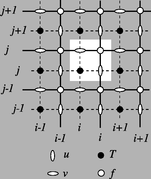scripts.get_examples.download_files(source_url, file_names, target_path)

Mirror file_names from source_url to target_path.

scripts.get_examples.main(target_path=None)

Get example scripts, example notebooks, and example data.

Copy the examples from the package directory and get the example data either from the package directory or from the Parcels website.

Indices and tables

• Index

• Module Index

• Search Page